Assessing engraftment extent with q2-FMT
Exploring the data
Access and summarize the study metadata
To begin our work with QIIME 2 and the tutorial data we will start by downloading the metadata, generating a summary, and exploring that summary.
First, download the metadata.
wget -O 'sample-metadata.tsv' \
  'https://q2-fmt.readthedocs.io/en/latest/data/tutorial/sample-metadata.tsv'
from qiime2 import Metadata
from urllib import request

url = 'https://q2-fmt.readthedocs.io/en/latest/data/tutorial/sample-metadata.tsv'
fn = 'sample-metadata.tsv'
request.urlretrieve(url, fn)
sample_metadata_md = Metadata.load(fn)
library(reticulate)

Metadata <- import("qiime2")$Metadata
request <- import("urllib")$request

url <- 'https://q2-fmt.readthedocs.io/en/latest/data/tutorial/sample-metadata.tsv'
fn <- 'sample-metadata.tsv'
request$urlretrieve(url, fn)
sample_metadata_md <- Metadata$load(fn)
md_url = 'https://qiime2-workshops.s3.us-west-2.amazonaws.com/itn-aug2024/sample-metadata-v3-q2-fmt.tsv'

sample_metadata = use.init_metadata_from_url('sample_metadata', md_url)sample-metadata.tsv| download
Next, we’ll get a view of the study metadata using QIIME 2. This will allow you to assess whether the metadata that QIIME 2 is using is as you expect. You can do this using the tabulate action in QIIME 2’s q2-metadata plugin as follows.
qiime metadata tabulate \
  --m-input-file sample-metadata.tsv \
  --o-visualization metadata-summ-1.qzv
import rachis.plugins.metadata.actions as metadata_actions
metadata_summ_1_viz, = metadata_actions.tabulate(
input=sample_metadata_md,
)metadata_actions <- import("rachis.plugins.metadata.actions")
action_results <- metadata_actions$tabulate(
input=sample_metadata_md,
)
metadata_summ_1_viz <- action_results$visualizationuse.action(
use.UsageAction(plugin_id='metadata', action_id='tabulate'),
use.UsageInputs(input=sample_metadata),
use.UsageOutputNames(visualization='metadata_summ_1')
)Access and summarize the feature table
The feature table will describe the amplicon sequence variants (ASVs) observed in each sample, and how many times each ASV was observed in each sample. The feature data in this case is the sequence that defines each ASV.
In this tutorial, we’re going to work specifically with samples that were included in the autoFMT randomized trial.
Lets generate and explore a summary of the feature table we will be using.
wget -O 'feature-table.qza' \
  'https://q2-fmt.readthedocs.io/en/latest/data/tutorial/feature-table.qza'
from qiime2 import Artifact

url = 'https://q2-fmt.readthedocs.io/en/latest/data/tutorial/feature-table.qza'
fn = 'feature-table.qza'
request.urlretrieve(url, fn)
feature_table = Artifact.load(fn)
Artifact <- import("qiime2")$Artifact

url <- 'https://q2-fmt.readthedocs.io/en/latest/data/tutorial/feature-table.qza'
fn <- 'feature-table.qza'
request$urlretrieve(url, fn)
feature_table <- Artifact$load(fn)
feature_table_url = 'https://qiime2-workshops.s3.us-west-2.amazonaws.com/itn-aug2024/autofmt-table.qza'

autofmt_table = use.init_artifact_from_url('feature-table', feature_table_url)qiime feature-table summarize \
--i-table feature-table.qza \
--m-metadata-file sample-metadata.tsv \
--o-feature-frequencies autofmt-feature-frequencies.qza \
--o-sample-frequencies autofmt-sample-frequencies.qza \
--o-summary autofmt-table-summ.qzvimport rachis.plugins.feature_table.actions as feature_table_actions
autofmt_feature_frequencies, autofmt_sample_frequencies, autofmt_table_summ_viz = feature_table_actions.summarize(
table=feature_table,
metadata=sample_metadata_md,
)feature_table_actions <- import("rachis.plugins.feature_table.actions")
action_results <- feature_table_actions$summarize(
table=feature_table,
metadata=sample_metadata_md,
)
autofmt_feature_frequencies <- action_results$feature_frequencies
autofmt_sample_frequencies <- action_results$sample_frequencies
autofmt_table_summ_viz <- action_results$summaryuse.action(
use.UsageAction(plugin_id='feature_table', action_id='summarize'),
use.UsageInputs(table=autofmt_table, metadata=sample_metadata),
use.UsageOutputNames(feature_frequencies='autofmt_feature_frequencies', sample_frequencies='autofmt_sample_frequencies', summary='autofmt_table_summ'),
)Selecting an Even Sampling Depth
Rarefying, rarefaction, and q2-boots
A first step in analyzing our microbiome feature table is to choose an “even sampling depth”, or the number of sequences that we should select at random from each of our samples to ensure that all samples are sequenced at equivalent depth or with equivalent effort. This processes is referred to as rarefying our feature table. Rarefying feature tables, or sampling them to a user-specified sampling depth and discarding samples with a total frequency that is less than the sampling depth, is a bit of a controversial topic because it throws away some of the data that was collected and is subject to biases as a result. Rarefaction differs in a subtle way from rarefying, in that it involves repeat sampling from the input feature table to a user-specified sampling depth. These concepts were recently discussed in Schloss (2024). In this tutorial, for the sake of time, we are going to focus our diversity analyses on rarefying (i.e., a single iteration of random sampling). To perform rarefaction-based diversity analysis with QIIME 2, refer to the q2-boots plugin Raspet et al. (2024).
Selecting an even sampling depth
To start our diversity analyses, we first need to determine what even sampling depth (or “rarefaction depth”) we want to select for computing our diversity metrics. Because most diversity metrics are sensitive to different sampling depths across different samples, it is common to randomly subsample the counts from each sample to a specific value. For example, if you define your sampling depth as 500 sequences per sample, the counts in each sample will be subsampled without replacement so that each sample in the resulting table has a total count of 500. If the total count for any sample(s) are smaller than this value, those samples will be dropped from the downstream analyses. Choosing this value is tricky. We recommend making your choice by reviewing the information presented in the feature table summary file. Choose a value that is as high as possible (so you retain more sequences per sample) while excluding as few samples as possible.
Open up the feature table summary that you previously created with either Galaxy or in your QIIME 2 container and we’ll discuss this as a group.
Alpha rarefaction plots
After choosing an even sampling depth, it’s helpful to see if your diversity metrics appear stable at that depth of coverage. You can do this for alpha diversity using an alpha rarefaction plot.
qiime diversity alpha-rarefaction \
  --i-table feature-table.qza \
  --p-metrics observed_features \
  --m-metadata-file sample-metadata.tsv \
  --p-max-depth 33000 \
  --o-visualization obs-features-alpha-rarefaction.qzv
import rachis.plugins.diversity.actions as diversity_actions
obs_features_alpha_rarefaction_viz, = diversity_actions.alpha_rarefaction(
table=feature_table,
metrics={'observed_features'},
metadata=sample_metadata_md,
max_depth=33000,
)builtins <- import_builtins()
diversity_actions <- import("rachis.plugins.diversity.actions")
action_results <- diversity_actions$alpha_rarefaction(
table=feature_table,
metrics=builtins$set(list('observed_features')),
metadata=sample_metadata_md,
max_depth=33000L,
)
obs_features_alpha_rarefaction_viz <- action_results$visualizationuse.action(
use.UsageAction(plugin_id='diversity', action_id='alpha_rarefaction'),
use.UsageInputs(table=autofmt_table, metrics={'observed_features'},
metadata=sample_metadata, max_depth=33000),
use.UsageOutputNames(visualization='obs-features-alpha-rarefaction'))Computing diversity metrics
The next step that we’ll work through is computing a series of common diversity metrics on our feature table.
We’ll do this using the q2-diversity plugin’s core-metrics action.
This action is a QIIME 2 Pipeline which combines over ten different actions in a single command.
Core diversity metrics
The core-metrics action requires your feature table and your sample metadata as input.
It additionally requires that you provide the sampling depth that this analysis will be performed at.
Determining what value to provide for this parameter is often one of the most confusing steps of an analysis.
Refer to the previous chapter for details.
Here we prioritize retaining samples and so we select a sampling depth of 10,000.
qiime diversity core-metrics \
  --i-table feature-table.qza \
  --p-sampling-depth 10000 \
  --m-metadata-file sample-metadata.tsv \
  --output-dir diversity-core-metrics
action_results = diversity_actions.core_metrics(
table=feature_table,
sampling_depth=10000,
metadata=sample_metadata_md,
)
rarefied_table = action_results.rarefied_table
observed_features_vector = action_results.observed_features_vector
shannon_vector = action_results.shannon_vector
evenness_vector = action_results.evenness_vector
jaccard_distance_matrix = action_results.jaccard_distance_matrix
bray_curtis_distance_matrix = action_results.bray_curtis_distance_matrix
jaccard_pcoa_results = action_results.jaccard_pcoa_results
bray_curtis_pcoa_results = action_results.bray_curtis_pcoa_results
jaccard_emperor_viz = action_results.jaccard_emperor
bray_curtis_emperor_viz = action_results.bray_curtis_emperoraction_results <- diversity_actions$core_metrics(
table=feature_table,
sampling_depth=10000L,
metadata=sample_metadata_md,
)
rarefied_table <- action_results$rarefied_table
observed_features_vector <- action_results$observed_features_vector
shannon_vector <- action_results$shannon_vector
evenness_vector <- action_results$evenness_vector
jaccard_distance_matrix <- action_results$jaccard_distance_matrix
bray_curtis_distance_matrix <- action_results$bray_curtis_distance_matrix
jaccard_pcoa_results <- action_results$jaccard_pcoa_results
bray_curtis_pcoa_results <- action_results$bray_curtis_pcoa_results
jaccard_emperor_viz <- action_results$jaccard_emperor
bray_curtis_emperor_viz <- action_results$bray_curtis_emperorcore_metrics_results = use.action(
use.UsageAction(plugin_id='diversity', action_id='core_metrics'),
use.UsageInputs(table=autofmt_table,
sampling_depth=10000, metadata=sample_metadata),
use.UsageOutputNames(rarefied_table='rarefied_table',
observed_features_vector='observed_features_vector',
shannon_vector='shannon_vector',
evenness_vector='evenness_vector',
jaccard_distance_matrix='jaccard_distance_matrix',
bray_curtis_distance_matrix='bray_curtis_distance_matrix',
jaccard_pcoa_results='jaccard_pcoa_results',
bray_curtis_pcoa_results='bray_curtis_pcoa_results',
jaccard_emperor='jaccard_emperor',
bray_curtis_emperor='bray_curtis_emperor'),
)diversity-core-metrics/rarefied_table.qza| download | viewdiversity-core-metrics/observed_features_vector.qza| download | viewdiversity-core-metrics/shannon_vector.qza| download | viewdiversity-core-metrics/evenness_vector.qza| download | viewdiversity-core-metrics/jaccard_distance_matrix.qza| download | viewdiversity-core-metrics/bray_curtis_distance_matrix.qza| download | viewdiversity-core-metrics/jaccard_pcoa_results.qza| download | viewdiversity-core-metrics/bray_curtis_pcoa_results.qza| download | viewdiversity-core-metrics/jaccard_emperor.qzv| download | viewdiversity-core-metrics/bray_curtis_emperor.qzv| download | view
As you can see, this command generates many outputs including both QIIME 2 artifacts and visualizations. We’ll work together on a guided exploration of these results.
Assessing engraftment extent with q2-FMT
When investigating FMTs, it is really important to understand the extent to which the recipient microbiome engrafted the donated microbiome. Without assessing engraftment extent, we can never fully understand the clinical outcomes of the study Figure 1.
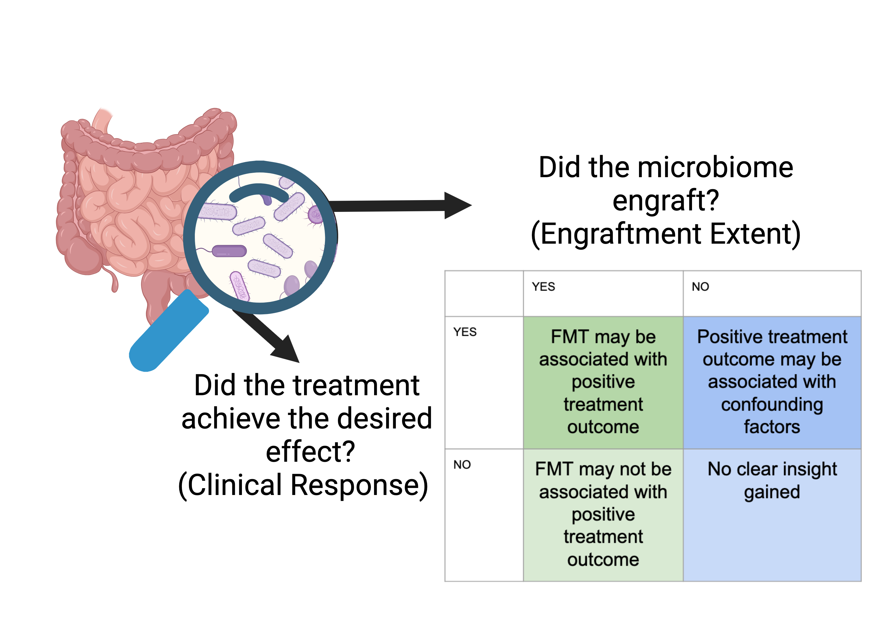
Figure 1:Created with BioRender.
Herman et al. (2024) Herman et al. (2024) defines three criteria that are important for understanding if a microbiome engrafted following FMT. These are:
- Chimeric Asymmetric Community Coalescence
- Donated Microbiome Indicator Features
- Temporal Stability.
q2-fmt is a QIIME 2 plugin that was designed to help you investigate all three of these criteria. For additional infomation, Here is a lecture video of Chloe Herman discussing the importance of assessing engraftment extent!
Chloe Herman at NIH presenting on assessing engraftment with q2-fmt!
In this tutorial we will be using q2-fmt to investigating all of these criteron.
Chimeric Asymmetric Community Coalescence
First, we’ll assess the distance to donor (using Jaccard distance) to see how the recipient’s distance to their donor sample changes following the FMT. Before continuing, think about what you might expect to see. Should you expect a recipient’s gut microbiome composition to become more or less similar to their donor after FMT? How quickly would you expect to see that change? What do you expect would happen a few months or years after the transplant?
qiime fmt cc \
  --i-diversity-measure diversity-core-metrics/jaccard_distance_matrix.qza \
  --m-metadata-file sample-metadata.tsv \
  --p-distance-to donor \
  --p-compare baseline \
  --p-time-column timepoints \
  --p-reference-column DonorSampleID \
  --p-subject-column PatientID \
  --p-filter-missing-references \
  --p-against-group 0 \
  --p-p-val-approx asymptotic \
  --o-stats jaccard-raincloud-stats.qza \
  --o-raincloud-plot jaccard-raincloud-plot.qzv
import rachis.plugins.fmt.actions as fmt_actions
jaccard_raincloud_stats, jaccard_raincloud_plot_viz = fmt_actions.cc(
diversity_measure=jaccard_distance_matrix,
metadata=sample_metadata_md,
distance_to='donor',
compare='baseline',
time_column='timepoints',
reference_column='DonorSampleID',
subject_column='PatientID',
filter_missing_references=True,
against_group='0',
p_val_approx='asymptotic',
)fmt_actions <- import("rachis.plugins.fmt.actions")
action_results <- fmt_actions$cc(
diversity_measure=jaccard_distance_matrix,
metadata=sample_metadata_md,
distance_to='donor',
compare='baseline',
time_column='timepoints',
reference_column='DonorSampleID',
subject_column='PatientID',
filter_missing_references=TRUE,
against_group='0',
p_val_approx='asymptotic',
)
jaccard_raincloud_stats <- action_results$stats
jaccard_raincloud_plot_viz <- action_results$raincloud_plotuse.action(
use.UsageAction('fmt', 'cc'),
use.UsageInputs(
diversity_measure=core_metrics_results.jaccard_distance_matrix,
metadata=sample_metadata,
distance_to='donor',
compare='baseline',
time_column='timepoints',
reference_column='DonorSampleID',
subject_column='PatientID',
filter_missing_references=True,
against_group='0',
p_val_approx='asymptotic'
),
use.UsageOutputNames(
stats='jaccard_raincloud_stats',
raincloud_plot='jaccard_raincloud_plot'
)
)In the resulting raincloud plot, we see that following cancer treatment (Timepoint 0-2) the recipients distance to donor is relatively high.This seems to be naturally resolving itself but after FMT intervention(Timepoint 3) the recipient’s microbiome looks more similar to the donated microbiome. We see some stability in this but by the last time point the recipient’s microbiome mostly looks unique from its donated microbiome.
Community Richness
While FMT research is still in its infancy, some early studies suggest that long-term, the emergence of “personalize microbiome” is common after FMT, but in some cases features of the donated microbiome are retained. Let’s investigate this idea in an exercise.
The community richness at each timepoint seems to be considerably variable and is never sigificantly higher than the baseline. It does look like after FMT intervention the community richness of the recipients is less variable but again it is not significantly higher than baseline. The last timepoint has the lowest community richness but there are only 3 subjects that were sampled that long after FMT. This makes it hard to tell if that is representative of the whole population or if those individuals where sampled that long after FMT because of complications.
Distance to Baseline
Developing a personalized microbiome following FMT intervention is expected. Although, there is no expected threshold for the length of time before personalization starts. It is important that the recipients microbiome doesn’t return to their baseline composition. qiime fmt cc can help us investigate this!
qiime fmt cc \
  --i-diversity-measure diversity-core-metrics/jaccard_distance_matrix.qza \
  --m-metadata-file sample-metadata.tsv \
  --p-distance-to baseline \
  --p-compare baseline \
  --p-time-column timepoints \
  --p-baseline-timepoint 0 \
  --p-subject-column PatientID \
  --p-filter-missing-references \
  --p-against-group 1 \
  --p-p-val-approx asymptotic \
  --o-stats baseline-jaccard-stats.qza \
  --o-raincloud-plot baseline-jaccard-raincloud-plot.qzv
baseline_jaccard_stats, baseline_jaccard_raincloud_plot_viz = fmt_actions.cc(
diversity_measure=jaccard_distance_matrix,
metadata=sample_metadata_md,
distance_to='baseline',
compare='baseline',
time_column='timepoints',
baseline_timepoint='0',
subject_column='PatientID',
filter_missing_references=True,
against_group='1',
p_val_approx='asymptotic',
)action_results <- fmt_actions$cc(
diversity_measure=jaccard_distance_matrix,
metadata=sample_metadata_md,
distance_to='baseline',
compare='baseline',
time_column='timepoints',
baseline_timepoint='0',
subject_column='PatientID',
filter_missing_references=TRUE,
against_group='1',
p_val_approx='asymptotic',
)
baseline_jaccard_stats <- action_results$stats
baseline_jaccard_raincloud_plot_viz <- action_results$raincloud_plotuse.action(
use.UsageAction('fmt', 'cc'),
use.UsageInputs(
diversity_measure=core_metrics_results.jaccard_distance_matrix,
metadata=sample_metadata,
distance_to='baseline',
compare='baseline',
time_column='timepoints',
baseline_timepoint='0',
subject_column='PatientID',
filter_missing_references=True,
against_group='1',
p_val_approx='asymptotic'
),
use.UsageOutputNames(
stats='baseline_jaccard_stats',
raincloud_plot='baseline_jaccard_raincloud_plot'
)
)Now lets look at the distance to their baseline. This will help us identify if the microbiome that emerges after FMT intervention is a unique personalized microbiome or if it is reverting to their baseline. Looking at this raincloud plot it looks like the microbiome always looks distinct from the baseline microbiome and that pattern continues all the way to the last timepoint. This probably indicates that the recipient microbiome following FMT is unique!
Proportional Engraftment of Donor Features (PEDF)
If you are interested in how many microbes from the donor engrafted in the recipient, Proportional Engraftment of Donor Features helps capture just that.
The above metrics capture how similar the recipient and donor microbiomes are. However, We want these microbiome to coalesce asymmetrically meaning that we want the donor’s features to be more prominment in the recipeint following FMT than baseline features. This metrics investigates this asymmetric colescence and captures how many donated features engrafted.
qiime fmt pedf \
  --i-table diversity-core-metrics/rarefied_table.qza \
  --m-metadata-file sample-metadata.tsv \
  --p-time-column timepoints \
  --p-reference-column DonorSampleID \
  --p-filter-missing-references \
  --p-subject-column PatientID \
  --o-pedf-dists pedf-dist.qza
pedf_dist, = fmt_actions.pedf(
table=rarefied_table,
metadata=sample_metadata_md,
time_column='timepoints',
reference_column='DonorSampleID',
filter_missing_references=True,
subject_column='PatientID',
)action_results <- fmt_actions$pedf(
table=rarefied_table,
metadata=sample_metadata_md,
time_column='timepoints',
reference_column='DonorSampleID',
filter_missing_references=TRUE,
subject_column='PatientID',
)
pedf_dist <- action_results$pedf_distspedf_dists, = use.action(
use.UsageAction('fmt', 'pedf'),
use.UsageInputs(
table=core_metrics_results.rarefied_table,
metadata=sample_metadata,
time_column='timepoints',
reference_column='DonorSampleID',
filter_missing_references=True,
subject_column='PatientID'
),
use.UsageOutputNames(
pedf_dists='pedf_dist'
)
)Now, we have our PEDF metrics and we want to visualize them.
Lets use qiime fmt heatmap.
qiime fmt heatmap \
  --i-data pedf-dist.qza \
  --o-visualization pedf-heatmap.qzv
pedf_heatmap_viz, = fmt_actions.heatmap(
data=pedf_dist,
)action_results <- fmt_actions$heatmap(
data=pedf_dist,
)
pedf_heatmap_viz <- action_results$visualizationuse.action(
use.UsageAction('fmt', 'heatmap'),
use.UsageInputs(
data=pedf_dists,
),
use.UsageOutputNames(
visualization='pedf-heatmap',
)
)Looking at this output, timepoint 0 seems to have very low proportional engraftment of donor strains. However, we can see that there is a a kind of bi-modal distribution at timepoint 1. Some of the samples have a relatively proportional engraftment of donor strains and some of them have a relatively low proportional engraftment of donor strains . At timepoint 3, we can see that there is less variation between recipients. This lines up pretty well with what we were seeing with the raincloud plot. This makes sense because they both are investigating Community Coalesense!
Note: you can also use qiime stats plot-rainclouds to visualize this data! This will create plots more similar to the ouput of qiime fmt cc above.
Permutation Test of PEDF
Now an important question to ask is:
“Is the overlap between features due to the FMT or are the similarities between these 2 microbiome by random chance”.
That’s where pedf-permutation-test comes in!
PEDF permutation testrandomizes the relationships between donors and recipients, to test whether the PEDS score between a recipient and their actual donor is significantly higher than PEDS scores between other recipients paired with random donors.
Note that we are testing this on an equal amount of pre-fmt and post FMT samples and this will likely lead to a more conservative global test results.
Alright, Lets take a look 👀.
qiime fmt pedf-permutation-test \
  --i-table diversity-core-metrics/rarefied_table.qza \
  --m-metadata-file sample-metadata.tsv \
  --p-time-column timepoints \
  --p-reference-column DonorSampleID \
  --p-filter-missing-references \
  --p-subject-column PatientID \
  --p-sampling-depth 10000 \
  --o-actual-sample-pedf actual-sample-pedf.qza \
  --o-per-subject-stats per-subject-stats.qza \
  --o-global-stats global-stats.qza
actual_sample_pedf, per_subject_stats, global_stats = fmt_actions.pedf_permutation_test(
table=rarefied_table,
metadata=sample_metadata_md,
time_column='timepoints',
reference_column='DonorSampleID',
filter_missing_references=True,
subject_column='PatientID',
sampling_depth=10000,
)action_results <- fmt_actions$pedf_permutation_test(
table=rarefied_table,
metadata=sample_metadata_md,
time_column='timepoints',
reference_column='DonorSampleID',
filter_missing_references=TRUE,
subject_column='PatientID',
sampling_depth=10000L,
)
actual_sample_pedf <- action_results$actual_sample_pedf
per_subject_stats <- action_results$per_subject_stats
global_stats <- action_results$global_statsactual_sample_pedf, per_subject_stats, global_stats = use.action(
use.UsageAction('fmt', 'pedf_permutation_test'),
use.UsageInputs(
table=core_metrics_results.rarefied_table,
metadata=sample_metadata,
time_column='timepoints',
reference_column='DonorSampleID',
filter_missing_references=True,
subject_column='PatientID',
sampling_depth=10000
),
use.UsageOutputNames(
actual_sample_pedf='actual_sample_pedf',
per_subject_stats='per-subject-stats',
global_stats='global-stats'
)
)We can now re-vizualize our heatmap and include these new stats that we created.
qiime fmt heatmap \
  --i-data actual-sample-pedf.qza \
  --i-per-subject-stats per-subject-stats.qza \
  --i-global-stats global-stats.qza \
  --o-visualization pedf-stats-heatmap.qzv
pedf_stats_heatmap_viz, = fmt_actions.heatmap(
data=actual_sample_pedf,
per_subject_stats=per_subject_stats,
global_stats=global_stats,
)action_results <- fmt_actions$heatmap(
data=actual_sample_pedf,
per_subject_stats=per_subject_stats,
global_stats=global_stats,
)
pedf_stats_heatmap_viz <- action_results$visualizationuse.action(
use.UsageAction('fmt', 'heatmap'),
use.UsageInputs(
data=actual_sample_pedf,
per_subject_stats=per_subject_stats,
global_stats=global_stats
),
use.UsageOutputNames(
visualization='pedf-stats-heatmap',
)
)We can see that there are many per-subject stats that where the simulated data(randomly paired recipients and donors) have higher PEDF than the true donor recipient pair but the majority of our comparisons are significant and globally are true pairs are significantly higher than our simulated donor recipient pairs.
Thats good news!
Proportional Persistence of Recipient Features (PPRF)
Proportional Persistence of Recipient Features (PPRF) investigates if there are any features from the recipients baseline that stick around after FMT intervention.
It is a very similar investigation to using fmt cc with the distance-to parameter set to baseline. This will again help us evaluate if a uniquew personalized microbiome is emerging or if the microbiome is reverting back to baseline.
qiime fmt pprf \
  --i-table diversity-core-metrics/rarefied_table.qza \
  --m-metadata-file sample-metadata.tsv \
  --p-time-column timepoints \
  --p-baseline-timepoint 0 \
  --p-filter-missing-references \
  --p-subject-column PatientID \
  --o-pprf-dists pprf-dist.qza
pprf_dist, = fmt_actions.pprf(
table=rarefied_table,
metadata=sample_metadata_md,
time_column='timepoints',
baseline_timepoint='0',
filter_missing_references=True,
subject_column='PatientID',
)action_results <- fmt_actions$pprf(
table=rarefied_table,
metadata=sample_metadata_md,
time_column='timepoints',
baseline_timepoint='0',
filter_missing_references=TRUE,
subject_column='PatientID',
)
pprf_dist <- action_results$pprf_distspprf_dists, = use.action(
use.UsageAction('fmt', 'pprf'),
use.UsageInputs(
table=core_metrics_results.rarefied_table,
metadata=sample_metadata,
time_column='timepoints',
baseline_timepoint='0',
filter_missing_references=True,
subject_column='PatientID'
),
use.UsageOutputNames(
pprf_dists='pprf_dist'
)
)This can also be viewed using fmt heatmap!
qiime fmt heatmap \
  --i-data pprf-dist.qza \
  --o-visualization pprf-heatmap.qzv
pprf_heatmap_viz, = fmt_actions.heatmap(
data=pprf_dist,
)action_results <- fmt_actions$heatmap(
data=pprf_dist,
)
pprf_heatmap_viz <- action_results$visualizationuse.action(
use.UsageAction('fmt', 'heatmap'),
use.UsageInputs(
data=pprf_dists
),
use.UsageOutputNames(
visualization='pprf-heatmap',
)
)From this visualization we can see that there is a relatively low presentage of persistant recipient features. Generally that’s a good sign of engraftment!
However, It looks like FMT.0035 has many persistant recipient features by timepoint 4. For an extra challenge go through our previous visualizations and see if you can identify any other signs of low engraftment extent!
Donated Microbiome Indicator Features
Another method that researchers commonly use to assess engraftment is donated microbiome indicator features
Currently, we do this by running ANCOMBC comparing the recipient at baseline to their donor. However because ancombc can not be run on dependent samples (i.e. a patient over time), we are not able to compare the baseline recipient to their donor because in this case they are the same patient.
However, some people investigate microbes that other papers reported as imported. We will investigate if the feature was in the donated microbiome and if the recipient recieved the feature.
This review reported that the class of Clostridia is correlated with positive health outcomes.
So here we are going to use q2-longitudinal to track the relative abunadnce of Clostridia over time. This will help us identify if the donated microbiome had the previously reported feature and if the recipients recieve this feature.
wget -O 'taxonomy.qza' \
  'https://q2-fmt.readthedocs.io/en/latest/data/tutorial/taxonomy.qza'
url = 'https://q2-fmt.readthedocs.io/en/latest/data/tutorial/taxonomy.qza'
fn = 'taxonomy.qza'
request.urlretrieve(url, fn)
taxonomy = Artifact.load(fn)
url <- 'https://q2-fmt.readthedocs.io/en/latest/data/tutorial/taxonomy.qza'
fn <- 'taxonomy.qza'
request$urlretrieve(url, fn)
taxonomy <- Artifact$load(fn)
taxonomy_url = 'https://qiime2-workshops.s3.us-west-2.amazonaws.com/itn-aug2024/taxonomy.qza'

taxonomy = use.init_artifact_from_url('taxonomy', taxonomy_url)Lets use this Taxonomy to collapse our table at level three or Class.
qiime taxa collapse \
  --i-table feature-table.qza \
  --i-taxonomy taxonomy.qza \
  --p-level 3 \
  --o-collapsed-table collapsed3-table.qza
import rachis.plugins.taxa.actions as taxa_actions
collapsed3_table, = taxa_actions.collapse(
table=feature_table,
taxonomy=taxonomy,
level=3,
)taxa_actions <- import("rachis.plugins.taxa.actions")
action_results <- taxa_actions$collapse(
table=feature_table,
taxonomy=taxonomy,
level=3L,
)
collapsed3_table <- action_results$collapsed_tablecollapsed3_table, = use.action(
use.UsageAction('taxa', 'collapse'),
use.UsageInputs(
table=autofmt_table,
taxonomy=taxonomy,
level=3
),
use.UsageOutputNames(
collapsed_table='collapsed3-table'
)
)Let’s transform this feature-table into relative frequency feature table. This will allow us to look at relative frequency instead of raw counts that can be misleading.
qiime feature-table relative-frequency \
  --i-table collapsed3-table.qza \
  --o-relative-frequency-table collapsed3-table-rf.qza
collapsed3_table_rf, = feature_table_actions.relative_frequency(
table=collapsed3_table,
)action_results <- feature_table_actions$relative_frequency(
table=collapsed3_table,
)
collapsed3_table_rf <- action_results$relative_frequency_tablecollapsed3_table_rf, = use.action(
use.UsageAction('feature_table', 'relative_frequency'),
use.UsageInputs(
table=collapsed3_table
),
use.UsageOutputNames(
relative_frequency_table='collapsed3-table-rf'
)
)Now we are ready to use q2-longitudinal to track our previously identified feature
Tracking Features with q2-longitudinal
qiime longitudinal linear-mixed-effects \
  --m-metadata-file sample-metadata.tsv collapsed3-table-rf.qza \
  --p-state-column day-relative-to-fmt \
  --p-group-columns autoFmtGroup \
  --p-individual-id-column PatientID \
  --p-metric 'k__Bacteria;p__Firmicutes;c__Clostridia' \
  --o-visualization lme-clostridia-treatmentVScontrol.qzv
from rachis import Metadata
import rachis.plugins.longitudinal.actions as longitudinal_actions
md_collapsed3_table_rf_md = collapsed3_table_rf.view(Metadata)
merged_collaped3_rf_md = sample_metadata_md.merge(md_collapsed3_table_rf_md)
lme_clostridia_treatmentVScontrol_viz, = longitudinal_actions.linear_mixed_effects(
metadata=merged_collaped3_rf_md,
state_column='day-relative-to-fmt',
group_columns='autoFmtGroup',
individual_id_column='PatientID',
metric='k__Bacteria;p__Firmicutes;c__Clostridia',
)longitudinal_actions <- import("rachis.plugins.longitudinal.actions")
md_collapsed3_table_rf_md <- collapsed3_table_rf$view(Metadata)
merged_collaped3_rf_md <- sample_metadata_md$merge(md_collapsed3_table_rf_md)
action_results <- longitudinal_actions$linear_mixed_effects(
metadata=merged_collaped3_rf_md,
state_column='day-relative-to-fmt',
group_columns='autoFmtGroup',
individual_id_column='PatientID',
metric='k__Bacteria;p__Firmicutes;c__Clostridia',
)
lme_clostridia_treatmentVScontrol_viz <- action_results$visualizationmd_collapsed3_table_rf= use.view_as_metadata(
'md_collapsed3_table_rf',
collapsed3_table_rf)
merged_collaped3_rf = use.merge_metadata(
'merged_collaped3_rf',
sample_metadata,
md_collapsed3_table_rf)
use.action(
use.UsageAction('longitudinal', 'linear_mixed_effects'),
use.UsageInputs(metadata=merged_collaped3_rf,
state_column='day-relative-to-fmt',
group_columns='autoFmtGroup',
individual_id_column='PatientID',
metric='k__Bacteria;p__Firmicutes;c__Clostridia'),
use.UsageOutputNames(visualization='lme-clostridia-treatmentVScontrol')
)Looking at this it looks like both the control and FMT groups had Clostrida in relatively low abundances. Both Groups seems to have in increase in Clostrida over time, which is good becuase we know thats correlated with postive treament outcomes. However, there is no significant change between groups. This suggests that Clostrida is not a great donor indicator for this group of patients.
Check back soon for more updates on tracking donated microbiome indicator features using ANCOMBC2 which will allow for repeated sampling!
Feature Engraftment
Feature engraftment doesn’t “assess engraftment” of a recipient but instead investigates if there are features that engraft across all subjects. This will help researchers understand which features are sucessfully engrafting and help them decide which successfully engrafted features correlate with postive clinical outcome.
This could be utilized to help researchers decide on specified communities to donate (as opposed the black-box commmunity approach we have currently). This specified communities would be full of microbes that have successfully engraftment accross patients and are associated with postive clincal outcomes.
Since we previously looked at the Clostrida, lets continue look at how our classes engraft accross subjects.
Let’s take a look now and see if we have any features that are sucessfully engrafting accross subjects.
qiime fmt prdf \
  --i-table collapsed3-table.qza \
  --m-metadata-file sample-metadata.tsv \
  --p-time-column timepoints \
  --p-reference-column DonorSampleID \
  --p-subject-column PatientID \
  --p-filter-missing-references \
  --o-prdf-dists pfdf-dist.qza
pfdf_dist, = fmt_actions.prdf(
table=collapsed3_table,
metadata=sample_metadata_md,
time_column='timepoints',
reference_column='DonorSampleID',
subject_column='PatientID',
filter_missing_references=True,
)action_results <- fmt_actions$prdf(
table=collapsed3_table,
metadata=sample_metadata_md,
time_column='timepoints',
reference_column='DonorSampleID',
subject_column='PatientID',
filter_missing_references=TRUE,
)
pfdf_dist <- action_results$prdf_distsprdf_dist, = use.action(
use.UsageAction('fmt', 'prdf'),
use.UsageInputs(
table=collapsed3_table,
metadata=sample_metadata,
time_column='timepoints',
reference_column='DonorSampleID',
subject_column='PatientID',
filter_missing_references=True
),
use.UsageOutputNames(
prdf_dists='pfdf_dist'
)
)And again, Visualize the data using qiime fmt heatmap.
We are using the level-delimiter parameter here so that the taxonomic strings will only show the lowest relevant taxonomic level!
qiime fmt heatmap \
  --i-data pfdf-dist.qza \
  --p-level-delimiter ';' \
  --o-visualization feature-heatmap.qzv
feature_heatmap_viz, = fmt_actions.heatmap(
data=pfdf_dist,
level_delimiter=';',
)action_results <- fmt_actions$heatmap(
data=pfdf_dist,
level_delimiter=';',
)
feature_heatmap_viz <- action_results$visualizationuse.action(
use.UsageAction('fmt', 'heatmap'),
use.UsageInputs(
data=prdf_dist,
level_delimiter = ';',
),
use.UsageOutputNames(
visualization='feature-heatmap',
)
)Oh look! Clostridia seems to be a feature that consistantly engrafts from our donor! It seems like it doesnt engraft “better” than spontanous recover but it is a consistant engrafter. Firmicutes also seems to pretty consistently engraft but it is important to note that our N for this study is quite small. Bacilli seems to engraft sucessfully too but its also present before the FMT so its hard to tell if thats from the donor or just a common gut 🐛 bug!
Overall in this study it seems that we have Asymetric Chimeric Community Coalesense. We also have stability in our shift towards the donated microbiome as there are no signs that our subjects are reverting back to baseline. From these factors I would conclude that we have relatively high engraftment extent and clincal findings are probably due to FMT engraftment. I would love to see more donated microbiome indicator species to further support this claim!
- Schloss, P. D. (2024). Rarefaction is currently the best approach to control for uneven sequencing effort in amplicon sequence analyses. mSphere, 9(2), e0035423.
- Raspet, I., Gehret, E., Herman, C., Meilander, J., Manley, A., Simard, A., Bolyen, E., & Caporaso, J. G. (2024). Facilitating bootstrapped and rarefaction-based microbiome diversity analysis with q2-boots. arXiv [q-Bio.QM].
- Herman, C., Barker, B. M., Bartelli, T. F., Chandra, V., Krajmalnik-Brown, R., Jewell, M., Li, L., Liao, C., McAllister, F., Nirmalkar, K., Xavier, J. B., & Gregory Caporaso, J. (2024). Assessing Engraftment Following Fecal Microbiota Transplant. ArXiv, arXiv:2404.07325v1. https://www.ncbi.nlm.nih.gov/pmc/articles/PMC11042410/